Experience, Innovation and Productivity - Empirical Evidence from Italy's Slowdown

The criterion function depends on the Zs, namely variables correlated with the decision of
introducing innovations, such as R&D expenditure at the beginning of the sample period and the
other determinants of innovation, including age and the share of temporary workers.

To estimate the parameters δ' we observe that the expected value E(D₁)=P(D₁=1)=P(δ^,Z_it+ω_it>0)
is the probability of being an innovative firm. If the error term ωit is assumed with E(ωit) = 0 and
V(ωit ) = 1 the (first stage) estimation method applied is the probit maximum likelihood.

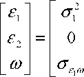
Usually equation (6) is estimated separately for the two regimes, whose idiosyncratic errors are
correlated with ωit, according to the covariance matrix:

Var

0

^σ2²

σ
ε₂

^σε1
^σε2
1

In this case we need to introduce corrections for the error conditional mean as in (8) and (8’):

where φ(∙) and Φ(∙) are, respectively, the standard normal density and cumulative distribution
functions. To calculate (8) and (8’) notice that we used the conditional distribution of ε given ω.
This is normal with mean E(εjit | ωit) = σεj1ωωit and variance V(εjit | ωit) = σj²-σ²εjω. Given (6)-(8’), our
specification becomes:

_{n l} ( Temporary       ΦδZ_it )

^{+β +γ}_lA^ge ^{+ μ}∣_:    ∖-2 ^{σ        +} U..

_     ,      ( Temporary         Φ(δZ_it )

+β₂ + γ₂ Age + μ₂∖-------H +σ_z> —-—i—+u2_i.

2     2 i 2                              ε₁ω                       2it

∖ L    Jit-2       ^1-φ(^δ Zit )

This system of equations can be estimated consistently with OLS (second stage) after substituting

the estimate of δ'Z in the correction terms (derived from first stage probit estimation).⁷

7

Building on Maddala (1983) we could simplify equation (9) simultaneously, adding the correction term, i.e. the sum
of (8) + (8’), for the whole sample:

12

<<   11   12   13   14   15   16   17   >>

More intriguing information