Country 1, ∆ Unemployment
Country 2, ∆ Unemployment

17
16
15
14
13
12
11
10
90
70
50
30
10
30
45
90 ʌ---ɔ
60 70
0.18
0.16
0.14
0.12
0.1
0.08
0.06
0.04
0.02
50
30
10
15
τ, (%)
30
45
s =L√Lw
τ, (%)
s =LZLw
60
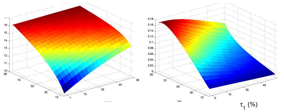
Figure 3: Change in unemployment [on the vertical axis] as a function of centrality and
size of the “bad” country 1 for a given change of b1 from 0.4 to 0.8.
countries 2 and 3.
Result 2b [Relative size and spill-overs]
The higher the relative size of country 1 the stronger is the increase in unemployment
rates in all countries due to a rise of country 1’s unemployment benefits.
Figure 3 shows that, at the benchmark value of τ = 30%, moving s1 from 0.1 to 0.9
increases the gradient of unemployment with respect to b1 from about 12 percentage points
to 16 in country 1 and from virtually zero to about 0.14 percentage points in countries
2 and 3. The logic for this result is similar to the one about centrality. When s1 is very
large, demand of firms in all countries depends mostly on country 1’s income. Hence,
variations in b1 have strong implications not only for country 1 but for the entire world.
If s1 is very small, the variation in b1 has implications only for a very small fraction of
global demand and therefore has little effect on unemployment rates world-wide.
Firm heterogeneity and the existence of fixed costs for foreign production have im-
portant implications for the quantitative impact of institutional changes in the directly
affected country 1 and in its trading partners. The reason is that a shortfall of income
in country 1 has first-order effects on firms of all productivities in country 1. However,
in countries 2 and 3, only firms with high productivity levels directly depend on country
1’s level of income as less inefficient firms do not engage in international trade and are
therefore sheltered from variation in country 1’s labor market institutions. This explains
why the quantitative impact of ∆b1 is much stronger in country 1 than in the rest of the
world.
23
More intriguing information
1. Surveying the welfare state: challenges, policy development and causes of resilience2. The name is absent
3. THE WAEA -- WHICH NICHE IN THE PROFESSION?
4. ROBUST CLASSIFICATION WITH CONTEXT-SENSITIVE FEATURES
5. The name is absent
6. The name is absent
7. The Importance of Global Shocks for National Policymakers: Rising Challenges for Central Banks
8. The name is absent
9. Structure and objectives of Austria's foreign direct investment in the four adjacent Central and Eastern European countries Hungary, the Czech Republic, Slovenia and Slovakia
10. The name is absent