PPP bl62

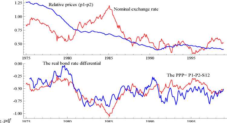
Figure 1: The graphs of price differential and the nominal exchange rate in logs (upper
panel), and the PPP together with bond rate differential (lower panel).
in Juselius (1995, 2006, Chapter 21) and Juselius and MacDonald (2004, 2006). An
important question is whether these persistent swings should be modelled as I(1) or
I(2). Since an I(2) variable typically exhibits smooth behavior, which can be difficult
to distinguish from an I(1) variable with a linear trend, the graphs of the differenced
data rather than the levels are often more informative about such I(2) behavior. Also,
inspecting the graph of the differenced process gives a first hint of whether the average
growth rate has been approximately zero or not, whether the growth rates have been
changing over the sample period, and whether there is significant mean reversion in
the differences.
Monthly differences are, however, often noisy and it is useful to apply a moving
average filter to the original data to single out the long-run movements from the tran-
sitory noise. This has been done in Figure 2, where we have graphed ∆(pp)t and ∆s12,t
filtered through a twelve-month moving average. The very persistent trending behav-
ior in ∆(pp~)t and ∆s12,t is apparent, suggesting that it may be useful to treat both
ppt and s12,t as I(2). We note that the inflation rate differentials exhibit more persis-
tent behavior than exchange rate changes. In the middle panel, we have graphed the
short-term interest spread and in the bottom panel the long-term interest rate spread.
In both cases, the long persistent swings suggest that these variables too exhibit I(2)
behavior.
Indeed, as we mentioned in the introduction, FGJ show that, under plausible as-
sumptions, the IKE model of swings in Frydman and Goldberg (2007) implies that the
exchange rate, relative goods prices, and interest rate spreads display I(2) behavior.
This is the case if the macroeconomic fundamentals on which market participants form
11
More intriguing information
1. CHANGING PRICES, CHANGING CIGARETTE CONSUMPTION2. Place of Work and Place of Residence: Informal Hiring Networks and Labor Market Outcomes
3. The name is absent
4. Surveying the welfare state: challenges, policy development and causes of resilience
5. Auctions in an outcome-based payment scheme to reward ecological services in agriculture – Conception, implementation and results
6. Who is missing from higher education?
7. The name is absent
8. The name is absent
9. Understanding the (relative) fall and rise of construction wages
10. Response speeds of direct and securitized real estate to shocks in the fundamentals