A MARKOVIAN APPROXIMATED SOLUTION TO A PORTFOLIO MANAGEMENT PROBLEM

The optimal investment- policy¹⁷ uɪ, called “cau-
tious”, is shown in Figure 22. The target is ⅛ =
1OO,OOO.

400

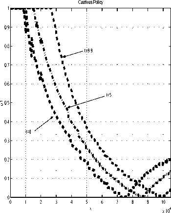
Fig. 22. A cautious policy.

350

300

cautious strategy

x₀=73500; Ex₁₀=99541

²⁵⁰ ^.....cautious'strategy...........■'

X0=60000;Exi0=84686 :   ^,'∙∙₄

median=86399 :         :

200 -........  (.........(.........(∙

150-∙

100-∙

50-

^x1-0^

∣ max expected value strategy ^:
∕x0=735OO)E<io=1672OO       ;

'I median= 84015     :         :

11111 111 I lJljijJL.JjjjjjJj-.iij-

0        0.2       0.4       0.6       0.8        1         1.2       1.4       1.6       1.8        2

x 10⁵

The solution is intuitively explicable: if there is a
shortage of funds, or time, the manager’s actions
become risky. In other words, the policy lines get-
higher and steeper as .τo falls. Also, for the part- of
the strategy graph where it- is impossible to meet
the target- xτ by investing in the riskless asset-
only (i.c., before each line hits 0.), each policy line
representing a later time dominates the lines that
correspond to earlier times.

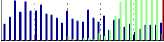
The usefulness of the cautious strategy for pension
fund management- can be assessed from Figure 23.

Fig. 23. A policy comparison.

Overall the cautious strategy appears an attrac-
tive portfolio management- policy. However, to use
it- for pension advertising, or for pricing the .Тю
“bond”, the objective function should reward the
manager for exceeding a target- (here, $100,000)
more than the square root- term¹⁸ .

An optimal control problem with g (ɪ (t ), и (t ), t) ≠
0 and s(X(T)) = e~^eτx(T} i.c., one in which
a combination of the final wealth and the util-
ity from consumption is maximised, can also be
solved using the above approximation method.

The cautious strategy was used to manage two
initial payments x₀ of $60,000 and $73,500. The
corresponding yield spreads arc represented by the
two central histograms in Figure 23. It- is easy to
see that the risk indices VaR and CVaR will be
very small for the first- outlay and virtually zero
for the second. For comparisons, the background
“back-t-o-back” histogram represents the result- of
managing the second payment- using the expected
value maximisation strategy. Oncc again we can
see that results worse than a “secure” investment
outcome ($99,215 in this ease) arc very probable.

6. CONCLUSION

A discretisation method useful for AIarkovian
approximations of finite-horizon continuous-time
stochastic optimal-control problems has been de-
scribed. An optimising algorithm has been devel-
oped (see [18] ) and applied to solve a portfolio
selection problem. For the calibrated models, an
overall agreement- between the analytical (where
obtainable) and approximating solutions was no-
ticed. However, a large variance of utility real-
isations was observed. It- was also noticed that
the variance diminished for constrained optimal
solutions.

In the example with variable volatility, no dif-
ference was reported in consumption patterns
between periods of low and high volatilities.

¹⁷Tho rest of the problem parameters are as before Lo.,
T = 10, u₂ = .02, r = .05, etc.

^lsFor example, (xτ - xτ)¹⁰ could be tried.

15