A MARKOVIAN APPROXIMATED SOLUTION TO A PORTFOLIO MANAGEMENT PROBLEM

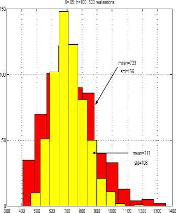
An impact- of the investment- constraint- on the
expected performance can be observed in more
detail in Figure 19. Two histograms of the dis-
counted total utility realisations arc presented.
The dark shadowed one corresponds to the un-
constrained policies (compare Figure 14). The
light- histogram represents the constrained pol-
icy performance. Evidently, the constrained policy
guarantees more “secure” performance (standard
deviation = 108 vis-à-vis 166 of the unconstrained
policy). However, the unconstrained policy brings
a (marginally) higher utility value. More compu-
tations of that kind would generate the “efficient-
boundary” .

utility

Fig. 19. Utility realisation distributions.

In a similar way, another portfolio problem, in
which some minimal (or maximal) consumption
rate is given could be solved.

5.3 Pension funds

A practical problem of financial engineering is one
in which an agent- pays an amount- .τo to a pension
fund, to be repaid by a quantity xτ at time T. The
latter is a result- of an investment- policy uι(.τ)
adopted by the fund’s manager.

The manager’s policy depends on his or her ob-
jective function, which could be the maximisation
of an expected value, the minimisation of risk to
obtain a target- amount-, etc. Oncc the objective
function is revealed, the manager’s policy can
be computed as a solution to a stochastic opti-
mal control problem associated with the objec-
tive function. The problem solution will routinely
comprise an optimal decision rule uι(.τ), U2(x)
and a Monte-Carlo simulated distribution of xγ∙
Knowing the former is crucial for the manager to
control the portfolio. The latter is “practical” in
that it- tolls the pension buyer what they can, or
should, expect- as xτ-

Knowing the distribution of xγ also helps the
manager. It- gives them an idea of what prob-
abilities, or risks, arc associated with obtaining
particular realisations of the objective function.
For example, the distribution may suggest- that,
for every .tq there is a probable terminal value
xτ, which the manager may choose to advertise
as the pension target-

Wc will first- solve a pension fund problem for
the expected value criterion, as follows. In (4),
set- <z(X(t),u(t),t) = 0, s(T(t)) = .τ(T) ¹²
and suppose that the management- fee is 2%.τ(t).
This means that we need to solve an optimisation
problem in uɪ(æ) with U∙₂(t) = .02.τ(t).

Using the Markovian approximation approach as
in Section 4.2, with the same model parameters
i.c., T = 10, r = .05, etc., generates a rather
trivial optimal strategy: t⅛_ιt = l,U2,t = ∙02.τ_f for
positive states and times. Applying the strategy to
different- initial outlays .f^,o generates the following
final fund yield spread and location measures¹³
at T = 10, see Figure 20.

The figure toll us, among other things, that an
initial deposit- of $40,000 corresponds to the ex-
pected pension value of about- $100,000. However,
the median fund’s yield for this objective function
is significantly below the mean. This indicates
that the fund distribution is skewed, which is evi-
dent- from Figure 21 (upper panel). The histogram
shows us too that the probability of earning less
than the “secure” revenue

40,000 cxp{(r — “management- fee") 10} = 53,994
is more than .5.¹⁴ It- is even fairly probable
(with probability >.4) to earn less than the initial
outlay .τo = 40,000. Evidently, using a policy
that maximises the expected yield is a very risky
strategy of managing a portfolio.

¹²Horo, the objective function is not HΛRΛ.

¹³Avoragod over 1000 realisations.

¹⁴To prove this and the subsequent claims integrate the
area under the histogram from zero to 53,994 and 40,000 ,
respectively.

<<   10   11   12   13   14   15   16   >>

More intriguing information