A MARKOVIAN APPROXIMATED SOLUTION TO A PORTFOLIO MANAGEMENT PROBLEM

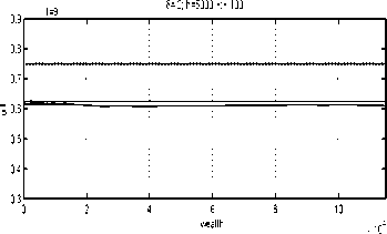
Fig. 9. Approximating strategies for t = 9
(5=.2).

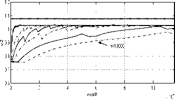
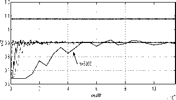
Fig. 11. Approximating strategies for t = 9
(5 = .05).

t=9                          δ=.1; h=10000 -:- 100

0.9 I-------------------------------------1-------------------------------------1-------------------------------------1-------------------------------------1-------------------------------------1---------------------------

0.8-...............i.................:.................i................∖................i...........-

0.7                                      ......^:.................

S 0.6-...............i.................:.................i................∖................i...........-

0.5-...............  :.................:................:................  -

0.4-...............i.................:.................i................∖................i...........-

0.₃∣-------------------------------------i-------------------------------------i-------------------------------------i-------------------------------------i-------------------------------------i---------------------------

0                 2                 4                 6                 8                 10

^wea∣^th                                           x 10⁴

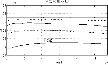
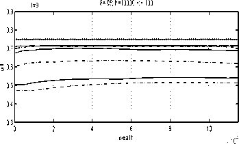
Fig. 10. Approximating strategies for t = 9
(5=.1).

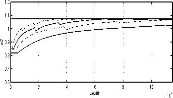
Fig. 12. Approximating strategies for t = 9
(5= .02 “small”).

Indeed, the gap between the optimal strategy and
the approximating strategies for t = O is narrow
for 5 = .2 and closes for 5 = .1 (for reasonably
small h) whereas, for t = 9, it narrows down only
for smaller 5s, see Figures 11 and 12. This is to
be expected because the optimal U2(T) = ∞,
and U2(T) = ∞ (see (32) and (30)), which is
impossible to reproduce numerically.

Figure 13 shows the wealth and strategy reali-
sations for 5 = .05 and h = 100. They look
very similar to the optimal ones in Figure 4. The
simulation of 2000 noise realisations and the appli-
cation of the approximating policy rules computed
for the same parameters (i.e., 5 = .05 and h =
100) resulted in the utility distribution (integrated
with the time simulation step equal to .025) shown
in Figure 14.

The mean discounted utility is J = 715.4 (98.9 %
optimal) and the corresponding standard devia-
tion is 161. However, the portfolio performance

<<   7   8   9   10   11   12   13   >>

More intriguing information