A MARKOVIAN APPROXIMATED SOLUTION TO A PORTFOLIO MANAGEMENT PROBLEM

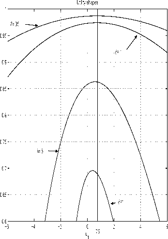
Fig. 6. Strategy convergence.

The vertical line t⅛=.75 shows where the utility
maximum “should” be, for it is known from Figure
2 that the optimal strategy is t⅛=.75, indepen-
dent of time. It is clear from the figure that the
discretised model strategy uχ_rι(δ) converges to the
optimal strategy as <) → 0. Again, any reasonable
approximation requires δ < .1.

Another point to remember is that the time step
δ should be large enough for the process to move
beyond the adjacent state i.e., δ∖f. ∣ > h. On the
other hand, as shown above, δ should be small for
high accuracy of the approximating solutions.

The convergence. There are various ways in
which the goodness of a numerical solution can
be evaluated. The most “objective” one would
perhaps be to look at the average discounted total
utility J generated by the application of an ap-
proximated optimal numerical solution to the con-
tinuous model. However, as evident from Figure 4,
the portfolio performance is very “volatile” and
the standard deviation of utility distribution is
large. Therefore, using J thus computed is difficult
to judge which solution is best.

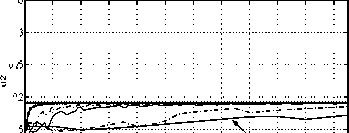
We will first evaluate the convergence by compar-
ing the approximating policy profiles (Figures 7 -
12), to the optimal ones (Figure 2).⁹ Then, we

⁹ Remember that because of the model re-scaling, if l'2
was linear (Figure 2) u2 will be horizontal.
will generate a few realisation profiles to compare
them to those of Figure 4 and, eventually, we will
compute the corresponding utility distribution.

S = .2; h=10000 -:- 100

0.81-

0.7

160

0.5-

0.4-

1          2         3         4         5         6         7         8         9         10        1 1

^wealth                                    x 10⁴

0.3

0.35

0.3

025

0.2

0.15

• h=10000

0.11-------------1-------------1-------------1-------------1-------------1-------------1-------------1-------------1-------------1-------------1-------------1_|

1          2         3         4         5         6         7         8         9         10        1 1

^wealth                                    χ10⁴

Fig. 7. Approximating strategies for t = 0
(5=.2).

Examine the policy rules shown in Figures 7 -
12. The bold dotted lines correspond to opti-
mal strategies (compare Figure 2). One can see
that the strategy convergence is more difficult
to achieve for later times (t = 9) than at the
beginning of the horizon (t = 0).

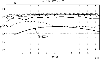
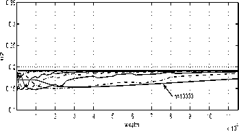
Fig. 8. Approximating strategies for t = 0
(5=.1).

<<   6   7   8   9   10   11   12   >>

More intriguing information