A MARKOVIAN APPROXIMATED SOLUTION TO A PORTFOLIO MANAGEMENT PROBLEM

3500

3000

2500

2000

1500

1000

500

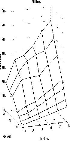
Number of maximisations

StateStep,00!03

■:.....«........

..⅛''

,o

,β

i'......;.........1

State Step .1125

: : .∙∙^s"'

.⅛S⅛⅛2.... jo≤

......'ʃ-

.......о............ : _:StateStep .15

1¹--------------------1---------------------1---------------------1---------------------1---------------------1--------------------1---------------------1---------------------1--------------------1---------------------₁

11 15 21 25 31 55 41 45 51 55 11

Numoer of Time Steps

Here, w is a one-dimensional standard Brownian
motion, and r, a, σ are constants with r < a and
σ > O. Symbol uɪ(t) denotes the fraction of the
wealth invested in the risky asset at t and U2{t)
is the consumption rate. The agent’s objective
is to find an optimal two-dimensional strategy
и = [ui(2t),[7₂(2t)], such that

O ≤ uɪ(t) ≤ 1, and U2{t) ≥ O, (27)

and such that maximises expected discounted
total utility

J(O, x(O); u) = IE

e-^βt[U₂{t)γdt I x(O)

(28)

Fig. 1. Computational complexity.

followed the optimal ones, see [8]. However, the
test problems were “easy” in that they contained
a quadratic cost component (they were not linear-
quadratic though). Here, the method will be used
to solve a classical portfolio selection problem
(see [2]) which is a generically stochastic and non
linear-quadratic problem.

given discount rate ρ > O and assuming that
[tf₂(t)]⁷ is the agent’s utility function. Here no
value is assigned to wealth at T while Xq is the
wealth at the initial time O. The problem to
maximise (28) subject to (26) is clearly one of the
class described in Section 2.1.

3.2 The Optimal Solution

The Hamilton-Jacobi-Bellman equation can be
solved for the optimal value function in the fol-
lowing form

3. A PORTFOLIO SELECTION MODEL

3.1 The Model

A simplified version of Merton’s [10] model of
optimal portfolio selection is analytically solved
in [2], pp. 160-161.

The stock portfolio consists of two assets, one
“risky” and the other “risk free”. If the price per
share of the risky asset p{t) changes according to
dp = p{ptdt + σdw)

while the price q per share for the risk free asset
changes according to

dq = qrdt

then the wealth x(t) at time t ∈ [O,T] changes
according to the following stochastic differential
equation

dx = (1 — u±)rxdt + u±x{adt + σdw) — U2dt.

(26)

Function g{τ) can be integrated and equals

p(τ) =

where

1~T
ρ-ι∕y

(1 — e

(g —^7)
1—i

1-7

(30)

(α — r)²
2σ²(l — 7)

+ r.

The optimal investment and consumption strate-
gies ûi and U2 can be computed as

n — r

Û1 = ɑ ʌ            31

σ²(l — 7)

lj2(τ,x) = [e^βτg(τ)]~ x. (32)

In this example, only JT₂ is a (linear) function
of wealth while ⅛ is constant. Notice also that
the above solution is “internal” in that both con-
straints (27) will be satisfied for some parameter
set. In particular ⅛ ≤ 1 if α — r ≤ σ²(l — 7).