4. A CALIBRATED MODEL
4
x 104
12∣-------
Portfolio Selection. Expected Values
4.1 The reference solution
10
Suppose an agent with an original wealth of ar0 =
$100,000 wants to maximise their satisfaction
during the coming T = 10 years. The instanta-
neous satisfaction is measured by ʌ/ɛ^(t)- The
risk free asset price drift is r = .05 and that of the
risky asset is a = .11 with the volatility σ = .4.
The agent’s discount rate is ρ = .11.
For these parameter values, the agent’s expected
discounted total utility is J = ρ(0)√100000 =
723.09. Figure 2 presents the optimal strategies;
the expected wealth and consumption rate time
profiles are shown in Figure 3.
Wealth
Consumption Rate
1
2
9 10
0
3 4 5 6 7 8
years
Fig. 3. Optimal expected wealth and consumption
rate time profiles.
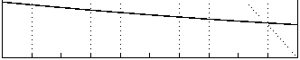
Optimal Strategies
1
0.8
0.6
0.4
0.2
0
0 2 4 6 8 10 12
4
x 104
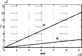
Fig. 2. Optimal (reference) strategies.
Optimal Realisations. Average Utility = 751
x 104
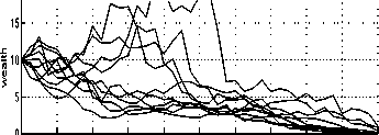
iF
0
0 1 2 3 4 5 6 7 8 9 10
□ 0.5-
6
Figure 4 shows ten wealth and strategy time
profiles, which correspond to ten noise realisations
dw(t), t ∈ [0,T], obtained from a random number
generator. The average total discounted utility of
these 10 portfolios is 751, which is more than the
theoretical J = 729. However, it is evident that
the optimal portfolios’ performance has a large
variance 8 .
0∣-------------------------------1-------------------------------1-------------------------------1--------------------------------1--------------------------------1--------------------------------1-------------------------------1-------------------------------1-------------------------------1-------------------------------
0 1 2 3 4 5 6 7 8 9 10
x 104
4
2
0 1 2 3 4 5 6 7 8 9 10
years
Fig. 4. Optimal wealth, investment and consump-
tion rate realisations.
0
4.2 Numerical Solutions
8 An estimate of the optimal utility standard deviation
was computed for the same integration parameter set as in
Section 4.2. (I.e., there were 600 noise realisations and the
integration step was .025.) The mean utility was 719.7,
which was 99.5 % of the theoretical expected optimal
performance; the corresponding standard deviation was
165.
The SOC Sol [18] suite of Matlab functions was
used to optimise a portfolio from Section 3. Most
of the problem transformation (e.g., from a con-
tinuous time and space formulation to a discrete
model) is taken care of by the software.
More intriguing information
1. The name is absent2. The name is absent
3. AN EMPIRICAL INVESTIGATION OF THE PRODUCTION EFFECTS OF ADOPTING GM SEED TECHNOLOGY: THE CASE OF FARMERS IN ARGENTINA
4. Restructuring of industrial economies in countries in transition: Experience of Ukraine
5. CONSUMER ACCEPTANCE OF GENETICALLY MODIFIED FOODS
6. Detecting Multiple Breaks in Financial Market Volatility Dynamics
7. Testing Gribat´s Law Across Regions. Evidence from Spain.
8. Multifunctionality of Agriculture: An Inquiry Into the Complementarity Between Landscape Preservation and Food Security
9. The name is absent
10. The name is absent