A MARKOVIAN APPROXIMATED SOLUTION TO A PORTFOLIO MANAGEMENT PROBLEM

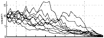
Approximated Realisations. Average Utility = 748

x 10⁴

ip

0          1          2         3         4         5         6         7         8         9

tions ∈ [159,162]).¹⁰ Averaging the utility over
more realisations and diminishing the simulation
step could help to improve the utility variance
estimate. However, the improvement would not be
substantial, as the portfolio pcrfomancc is highly
“volatile” whether optimal (Figure 4) or not (Fig-
ure 13).

5. PORTFOLIO MODEL MODIFICATIONS

0∣---------------------1---------------------1---------------------1---------------------1---------------------1---------------------1---------------------1---------------------1---------------------L

0          1          2         3         4         5         6         7         8         9

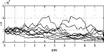
Fig. 13. Approximated wealth, investment and
consumption rate realisations.

Fig. 14. Utility realisation distribution.

5.1 Time Varying Parameters

Suppose now that the agent- expects the volatility
coefficient- σ to vary as follows
where σ = .4. This means that the volatil-
ity σ used in Sections 3 and 4 was an average
value. Now, the volatility will rise from 36.4 %
to 43.6 % in the middle of T, and then drop. The
agent- would like to know whether this information
should change their investment- strategy or not-.

Figure 15 reveals the modified strategy obtained
as a solution to the discrct-iscd portfolio problem
with ∂' = .05 and h = 500. As expected¹¹, the
agent- will invest- more (i.c., above .75) when the
volatility is low. The solution is “exact” in that we
can read how much one has to invest- at each time.
Interestingly, the optimal consumption strategy
remains unchanged.

The wealth and strategy sample paths for the
cosine volatility problem arc shown in Figure 16.
The discounted total utility is 664 (std=158).

In summary, the agent- should modify their in-
vestment- strategy once the information about- a
volatility scenario becomes available. In a similar
way, a portfolio problem with a time dependent-
interest- rate (or other parameters) can be solved.

as judged by index J for other approximating
rules (c.g., ∂' = .05, .02 and h = 500, 100) was
comparable (J ∈ [701, 720] with standard devia-
¹⁰Howovor, using ∂' = .5, h = 10000 that is clearly a “bad⁴’
policy, resulted in J = 124.13 with the standard deviation
equal 100.

¹¹ Soo footnote 19.

<<   8   9   10   11   12   13   14   >>

More intriguing information