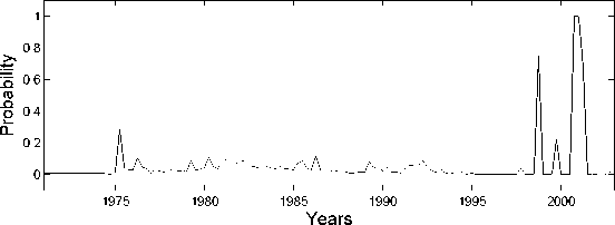
Temporal Distribution of Regime1

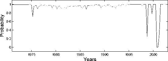
Temporal Distribution of Regime2

Figure 1: Germany, Fiscal Policy Rule, Temporal Distribution of Regime Probabilities, 1970-
2003.
between revenues/GDP and debt/GDP. These may easily be plotted using the estimated median
values of the coefficients for γB (StF = 1), γB (StF = 2) and the two constants. This delivers a
straight line in debt/output, revenue/output space for each of the two regimes. A graphical
representation is given in figure 3 and will be discussed in detail in section 2.4. In regime 1 we
observe larger values for the revenue/GDP ratio than in regime 2, when the debt/GDP ratio
exceeds a value of about 140 %. When looking at the data for Germany’s debt/output ratio, we
find values of almost 250 % toward the end of the sample8 . From this it follows that regime 1
leads to larger revenue/output ratios in comparison to regime 2 at the end of the sample, when
fiscal authorities have accumulated a substantial level of debt.
This shows that there seems to be a tendency toward a more sustainable fiscal policy in
Germany with respect to debt in the late 1990s. Nonetheless, this shift in fiscal policy behavior
is not permanent, as we observe fluctuations between the two regimes till the end of the sample
period in figure 1. The analysis suggests so far that German fiscal policy underwent changes
in its fundamentals, as the switch to regime 1 means a decrease in autonomous government
expenditures, as depicted by the constant, combined with a more reactive behavior to increases
in government debt.
8 One should note that we divide total debt by quarterly GDP. Therefore, the debt/output ratio on an annual
basis would be four times smaller.
More intriguing information
1. Publication of Foreign Exchange Statistics by the Central Bank of Chile2. Human Resource Management Practices and Wage Dispersion in U.S. Establishments
3. Experimental Evidence of Risk Aversion in Consumer Markets: The Case of Beef Tenderness
4. THE ANDEAN PRICE BAND SYSTEM: EFFECTS ON PRICES, PROTECTION AND PRODUCER WELFARE
5. The name is absent
6. Discourse Patterns in First Language Use at Hcme and Second Language Learning at School: an Ethnographic Approach
7. Reputations, Market Structure, and the Choice of Quality Assurance Systems in the Food Industry
8. Party Groups and Policy Positions in the European Parliament
9. The Advantage of Cooperatives under Asymmetric Cost Information
10. A Study of Prospective Ophthalmology Residents’ Career Perceptions