Second Order Filter Distribution Approximations for Financial Time Series with Extreme Outlier

J.Q. Smith and Antonio Santos

treme. We measured this phenomena by counting the number of states for which
the distribution was approximated using a small number of distinct particles. We
ran the first order APF and analysed the distribution of the states for which the
distance between the highest particle and the lowest was less than 0.2. In Figure 2
and the bottom row of Table 1 it can be seen that there were many such states in

the first order APF but not in the second.

1

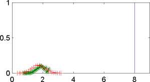
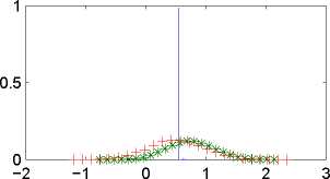
Figure 3: Histograms of the smoothing (+) distribution, first order filter distribution
(-) and second order filter distribution(*). Each figure correspond to the respective sub-
sample and the states analysed are for each sub-sample α ₁₀₈, α₈₅₂ and α₁₆₄₆, respectively.

Finally in Figure 3, we compared the filter distribution using a first and second
order approximation with the smoothing distribution associated with a given state.
We obviously expected that the filter distributions to be different from the smooth-
ing distributions because they were built from different information sets. However,
the smoothing distribution is able to give us an initial idea regarding the location
and dispersion of the filter distribution. In fact, it turns out that in the second
and third sub-samples, these states were very near the end of the sample, which
means that there was only a small difference between information sets. For exam-

G.E.M.F - F.E.U.C.

<<   15   16   17   18   19   20   21   >>

More intriguing information