The name is absent

which means a* = 0 or:

And so the steady-state Pareto-optimal solution is:

(nɪ + n2) b + ρ -  ₂5)

(x²(t)+1)

2x(t) (eɪnɪ + n2c2)

3.2 Graph and Analysis of the Steady-state Dynamic Pareto-
optimal Solution

This solution can be plotted in the (x,a)-plane together with the phase plot for
the steady-states of the lake when dx/dt = 0, given by equation (3). The inter-
section of the two curves gives society’s optimal phosphorous loading solution.
Using the hysteretic lake value b = 0.6, ρ = 0.03, nɪ = 2, n₂ = 2, c₁ = 0.2 and
c2 = 2, the graphs intersect at (x^*, a^*) = (0.3472, 0.1007), as shown in Figure 1
below, thus giving us the Pareto-optimal steady-state equilibrium. Note that
this result is below the point at which the lake flips from an oligotrophic to a
eutrophic state, i.e. for the selected constants, society prefers an oligotrophic
lake.

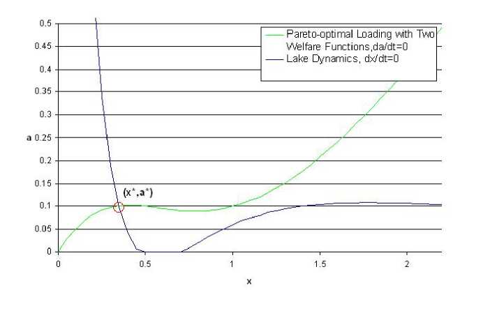
Figure 1: Pareto-optimal Loading with Two Welfare Functions

<<   9   10   11   12   13   14   15   >>

More intriguing information