approximated as
1K
hlog I det J D≈ K £log I det Jk I = E, (7)
k=1
where Jk denotes the value of J for the k-th training pattern,
and K is the number of training patterns.
E is the objective function that is maximized during
training. This is a function of the Jacobians Jk . Its gra-
dient is computed by backpropagating through an auxiliary
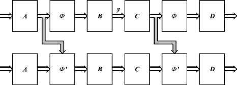
network that computes Jk . Figure 2 shows an example of
such a network, for the case of F and ψi blocks each im-
plemented through an MLP with a single, nonlinear hidden
layer, and with linear output units.

Fig. 2. Network for computing the Jacobian.
The upper part of the figure depicts the network of Fig.
1, shown in a different form. Block A multiplies the input
pattern by the input weight matrix of the F module. Its out-
puts are the input activations of the hidden units of F. The
leftmost Φ block applies the nonlinear activation functions
of those hidden units to each of those activations, yielding
the vector of output activations of the hidden units. Block B
then multiplies these activations by the output weight ma-
trix of F, yielding the vector of extracted components, y.
Blocks C, rightmost Φ and D represent, in a similar fash-
ion, the ψi modules (which, taken together, form a single-
hidden-layer MLP).
The lower part of the figure is the part that computes the
Jacobian proper. It propagates matrices, instead of vectors
(this is depicted in the figure by the 3D arrows). Its input is
the n × n identity matrix. All its blocks perform products
by matrices. Matrices A, B, C and D are the same as in
the upper part (each without the column corresponding to
bias terms), and the two Φ0 blocks correspond to diagonal
matrices, in which each diagonal element is the derivative
of the activation function of the corresponding hidden unit.
The gray arrows transmit the hidden units’ activations to
the lower part, to allow it to compute these derivatives. The
output of the lower part is the Jacobian corresponding to the
pattern that is presented at the input of the upper part.
For computing the gradient of E relative to the network’s
weights, we backpropagate through this network, inputting
into the lower part, on the right hand side, the value
J = J ~1) T ■ (8)
Nothing is input into the upper part, because E doesn’t de-
pend on z. Backpropagation must be performed along all
information transfer paths (i.e. along both the white and the
gray arrows). More details can be found in [8].
An important remark is that the values of the compo-
nents of the gradient of E vary widely during the training.
It is very important to use a fast training procedure, which
can deal with such variations effectively. We have used, in
all tests with MISEP, the adaptive step sizes technique with
error control described in [10], with very good results.
Matlab-compatible code implementing MISEP with a
structure based on MLPs is available at
http://neural.mesc-id.pt/~lba/ICA/MIToolbox.html.
3. LEARNING SPEED
The way in which both INFOMAX and MISEP extract in-
dependent components can be described as trying to make
the distribution of z become uniform. Since z is bounded to
a hypercube, its distribution being uniform implies that its
components zi will be mutually independent. Since each yi
is univocally related to the corresponding zi , the yi will also
be independent.
Intuitively speaking, the uniformization of the distribu-
tion of z is achieved in the following way: For each pattern
o that is presented at the input, the corresponding output z is
computed, and a ”spreading force” is applied, at that point,
to the mapping between o and z. If there is a region where
the output patterns z are more densely packed, more spread-
ing force is applied in that region, tending to uniformize the
output distribution.
Given this description, one would expect the training
to perform a relatively smooth uniformization of the out-
put distribution: The regions of higher density would be ex-
pected to simply spread until the density becomes uniform.
This is not what happens, however. The reason is that the
mapping between o and z is constrained by the structure of
the network that implements it. The network may not be
able to simply spread a region without impairing the uni-
formization that has already been achieved in other regions.
This is especially true if the F block is implemented
with non-local units, as is the case with an MLP. This phe-
nomenon has been observed by us in practice: sometimes,
some regions of relatively high density, in the output space,
remain for quite a long time during learning. During that
time, learning proceeds quite slowly. Apparently the MLP
needs to simultaneously adjust several of its units in order
to be able to expand these high density regions without af-
fecting what has already been done in other regions of the
output space.
More intriguing information
1. The name is absent2. Modelling the health related benefits of environmental policies - a CGE analysis for the eu countries with gem-e3
3. Wage mobility, Job mobility and Spatial mobility in the Portuguese economy
4. EFFICIENCY LOSS AND TRADABLE PERMITS
5. The name is absent
6. Comparison of Optimal Control Solutions in a Labor Market Model
7. The Triangular Relationship between the Commission, NRAs and National Courts Revisited
8. NATIONAL PERSPECTIVE
9. KNOWLEDGE EVOLUTION
10. Inflation Targeting and Nonlinear Policy Rules: The Case of Asymmetric Preferences (new title: The Fed's monetary policy rule and U.S. inflation: The case of asymmetric preferences)