This raised the question of whether using a network of
local units would be able to yield a significantly faster train-
ing. The following section shows experimental results that
confirm that this is indeed true.
4. COMPARISON BETWEEN LOCAL AND
NONLOCAL NETWORKS
We performed tests in which we compared, on the same
nonlinear ICA problems, networks in which the F module
had an MLP structure and networks in which that block was
based on radial basis function (RBF) units, which have a
local character. In the MLP-based case, that module was
formed by an MLP with a single hidden layer of sigmoidal
units and with linear output units. All hidden units received
all the inputs. Half of the hidden units were connected to
each of the module’s outputs. The network also had di-
rect connections between inputs and outputs (these direct
connections can be seen as implementing a linear mapping
which is modified, in a nonlinear way, by the hidden layer
units). This structure was chosen because it was the one
which showed to be most effective, in our previous experi-
ence with MISEP. All the network’s weights were trained
using the gradient of the objective function.
In the RBF-based implementation, the F block had a
hidden layer with Gaussian radial basis function units and a
linear output layer, and also had direct connections between
its input and output units. Again, these direct connections
can be seen as implementing a linear mapping, which is then
modified, in a nonlinear way, by the RBF units. The RBF
units’ centers and radiuses were trained in an unsupervised
manner, as described in [11]. Only the weights connecting
the hidden units and the input units to the output ones were
trained based on the gradient of the objective function.
The ψi modules were implemented in the same way in
both cases. Each of them consisted of an MLP with two
hidden units (with scaled arctangent activation functions)
and with a single linear output unit. Each of these networks
has a single input and a single output, and therefore the MLP
structure doesn’t give it any non-local character. All the
weights of these modules were trained based on the gradient
of the objective function.
Although our main purpose was to study the nonlinear
ICA operation itself, the tests were performed in a way that
allowed the approximate recovery of the original sources.
As discussed elsewhere [8], this is possible when the non-
linear mixture is smooth, requiring adequate regularization
of the separation transformation performed by the network.
As in previously reported tests, the MLP-based networks
didn’t require any explicit regularization, the inherent regu-
larization performed by MLPs being sufficient. The RBF-
based networks required explicit regularization, however.
This was implemented in the form of weight decay, applied
only to the weights linking the hidden units of module F
to its output units. The decay parameter was adjusted, in
preliminary tests, to a value that allowed the approximate
separation of the sources.
These networks were tested with two artificial mixtures:
a mixture of two supergaussian sources, and a mixture of
a supergaussian and a subgaussian, bimodal source. The
stopping criterion that was used in the training was based
on the value of the objective functionE. Since this function
is an estimate of the mutual information I(y) - apart from
an additive constant, cf. (4,6,7) - this stopping criterion de-
manded the same separation quality (as measured by mutual
information) for both implementations.
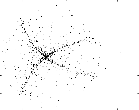
Figure 3 shows the nonlinear mixture of supergaussian
components that was used in the tests. Figures 4 and 5 show
the results of ICA performed by the MLP-based and the
RBF-based implementations, respectively. It is interesting
to note that the two results were almost identical, except for
a scaling of the components.
0.15
0.1
0.05
0
-0.05
-0.1

-0.05
0.05
0.15
Fig. 3. Mixture of supergaussian sources.
Figure 6 shows the nonlinear mixture of a supergaus-
sian and a subgaussian. Figures 7 and 8 show the results
of ICA performed by the MLP-based and the RBF-based
implementations, respectively.
Table 1 shows the means and standard deviations of the
numbers of epochs required to reach the stopping criterion,
for both kinds of networks. One epoch took approximately
the same time in both kinds of network. It is clear that
the RBF-based implementations trained much faster, and
showed a much smaller oscillation of training times2. This
confirms our interpretation that the cause for the relatively
2 Strictly speaking, the times involved in the unsupervised training of
the RBF units’ centers and radiuses should be added to the RBF networks’
results. However, these times were much shorter than those involved in the
gradient-based optimization, and thus were not considered here.
More intriguing information
1. National curriculum assessment: how to make it better2. Are class size differences related to pupils’ educational progress and classroom processes? Findings from the Institute of Education Class Size Study of children aged 5-7 Years
3. The name is absent
4. The Role of area-yield crop insurance program face to the Mid-term Review of Common Agricultural Policy
5. Firm Creation, Firm Evolution and Clusters in Chile’s Dynamic Wine Sector: Evidence from the Colchagua and Casablanca Regions
6. Artificial neural networks as models of stimulus control*
7. Implementation of the Ordinal Shapley Value for a three-agent economy
8. Subduing High Inflation in Romania. How to Better Monetary and Exchange Rate Mechanisms?
9. The name is absent
10. The effect of classroom diversity on tolerance and participation in England, Sweden and Germany