The name is absent

IOl

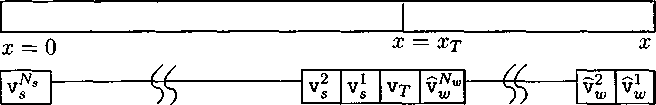
Figure 4.1: Schematic of the strong-weak model for a uniform fiber, along with its spatial
discretization to illustrate the ordering of compartments

absolute and relative voltages at the transition point:

V_τ(t) = V_s(x_τ,t) = V_w(x_τ,t), υ_τ(t) = V_τ(t) - V_τ.

(4.1)

It will be computationally advantageous to work with voltages with respect to rest.

The strong fiber obeys the nonlinear cable equation, while the weak fiber obeys
the quasi-active version of this PDE. Hence, using the cable equation from §2.3.1, we
write the strong-weak system as

ɪ                c                    F_c

G_jC_rric)fV_s _ ɑ ∂χχX_s G G_sc(x)(v_s   E_c ) ɪɪ scf Is(Vs> ^∙> t)

0 < X < xτ, 0 < t,

∂_tw_scf

G) cf ,oo('ʊ s)    'G'scf

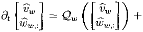
xτ < x < P, 0 < t,

(4.2)

(4.3)

(4.4)

where v_w and ω,,_jc denote the linearized weak voltage and gating variables, Φ denotes
the ionic current function, I_s and denotes the inputs to the strong fiber, I_w denotes
the linearized inputs to the weak fiber, and Q_w is the quasi-active operator, as in