Figure 8: The property-retrieval strategy

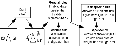
Figure 9: The find-fact-on-feedback strategy
general rule that wants to create a new example. The second
strategy, find-fact-on-feedback, is demonstrated in figure 9.
If the model has decided it will retrieve the weights, it still
cannot predict an answer, because it doesn’t even know what
the available answers are. So a “I don’t know” production
fires, after which the environment hopefully will give some
feedback. Suppose we have a child facing a real beam, it can
see that the answer is “left”. The strategy then tries to find
some fact in declarative memory that can help to predict the
answer. This can be an arbitrary fact, but since “beam”, “2”,
“3” and “left” are all part of the goal, ACT-R ensures that
facts containing these elements, or having associations with
them, are likely candidates. So 3 is-greater-than 2 is a possi-
ble candidate, particularly if there is already an association
between beam and greater-than, i.e. the child already knows
that beams have something to do with the fact that one thing
is greater than another.
Results
Simulations of the model, discussed in detail in Taatgen
(1996), show that it can indeed infer the correct rules for the
beam task. If the model already has an association between
beams and weight and between beams and greater-than, the
correct rules can be inferred using only a few examples. If
the model has no prior associations at all, it may need as
much as 40 examples, and in some runs it cannot even find
the correct rules at all.
When the model starts out with a wrong hypothesis, for
example that the labels have to be used to predict the out-
come, it shows a behavior similar to the explore-impasse-
insight-execute scheme: it first learns a lot of irrelevant rules
to predict the answer using the labels, then reaches a stage in
which it tries to explain a single example over and over again
but fails in doing this, after which it rejects the rule that
examines the labels, creates a rule that examines the weights,
and quickly derives the rest of the rules needed within a few
trials. Figure 10 shows an estimation of the time spent at

Figure 10: Estimated time spent at each trial before and after
the “insight” trial
each trial before and after the moment the model creates the
rule to examine weight instead of label.
Same model, other task: discrimination-shift
Another interesting property of the model is that its rules are
general, and can be applied to other tasks. A task that can be
modeled using the same production rules is discrimination-
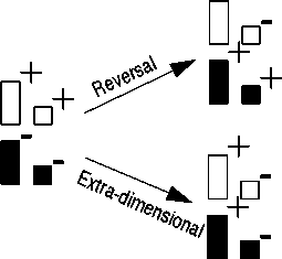
shift learning (Kendler & Kendler, 1959). Figure 11 shows
an example of this task: subjects have to learn to discrimi-
nate the four stimuli in two reinforcement categories, for
example white is positive and black is negative. After the
subjects has made 10 consecutive correct predictions, the
reinforcement scheme is changed: either a reversal-shift, in
which all stimuli that received previous positive reinforce-

Figure 11: Example of discrimination-shift learning
More intriguing information
1. Return Predictability and Stock Market Crashes in a Simple Rational Expectations Model2. Nonparametric cointegration analysis
3. The name is absent
4. Expectations, money, and the forecasting of inflation
5. The name is absent
6. Equity Markets and Economic Development: What Do We Know
7. Update to a program for saving a model fit as a dataset
8. The Evolution
9. Governance Control Mechanisms in Portuguese Agricultural Credit Cooperatives
10. A Unified Model For Developmental Robotics