TOMOGRAPHIC IMAGE RECONSTRUCTION OF FAN-BEAM PROJECTIONS WITH EQUIDISTANT DETECTORS USING PARTIALLY CONNECTED NEURAL NETWORKS

Learning and Nonlinear Models - Revista da Sociedade Brasileira de Redes Neurais, Vol. 1, No. 2, pp. 122-130, 2003
© Sociedade Brasileira de Redes Neurais

where each output yj is connected to the input xi with a weight wji. Comparing this expression with equation (8), allows one to
rewrite the backprojections in terms of synaptic weights where each pixel in the final image are fully connected by weights wij
to all pixels of q(s,θ). Index j enumerates all M pixels in the final image f(r,θ) while index i enumerates all N pixels in q(s,q):

1^N1^N

^f ( r^{φ φ}) = y_j =  ∑ wiX = ∑ wi_iq (^s, θ)

Ki=1         Ki=1

(10)

Note that some weights will be unity and others will be zero. To reduce memory usage and improve speed the null weights can
be purged yielding a partially connected neural network.

Equation (8) can be slightly modified to take into account the fan-beam geometry (4 ) [8]:

1 K 1   r cos(βi- φ)

^f (^r,^φ = K ∑ W ^q (—U—^β

(11)

The neural network can be easily modified to incorporate this new scenario. The only change needed is on the weights
values. Instead of unity their value should be given by

wji = U^-2

(12)

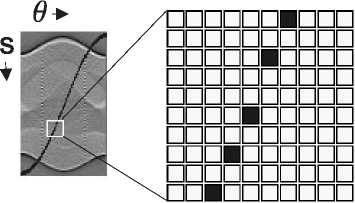
Figure 6: Zoom of part of the sinusoid, showing the points calculated according to the equation 4.

Another refinement to be incorporated in the reconstruction network is interpolation. When discretizing the calculated
value of s which is a function of the angle θ as expressed in (4) the nearest pixel is selected. This way only a few relevant
pixels in q(s,θ) will contribute to a given pixel in the final image. Figure 6 shows a zoomed view of the sinusoid relation in
q(s,θ) where significant space between adjacent pixels can be seen. To improve image quality, we use the interpolation method
[11,12] to make a good use of neighboring pixels. The procedure to obtain a linear interpolation is to compute a weighted
combination of the two adjacent pixels according to proximity of them to the sinusoid. Figure 7 illustrates the adjacent pixels
incorporated. Backprojection is then given by:

1^K

^f (^{r, φ}) = — ∑ [U_k q(_ ^s J^{, θ} ) + v_kq(P ^s 1^{, θ} )]

K k =1

(13)

where the calculated value of s is truncated downwards _sJ (floor of s) to the closest number in the discretized s axis, or
truncated upward Ps1 (ceil of s).

The weights ui and vi are calculated by

u_i =P s 1 - s = P s∣ - r cos(θ_i - φ)

and

v_i = s - _sJ = r cos(θ_i - φ) - _s J

(14)

(15)

126